DC Servo Motor Control: Parameter Extraction, Controller Architecture

Some methods for model parameter extraction necessary for accurate control of DC servo motor, controller architectures, as well as existing hardware that deploys some of the technology will be reviewed.

Controller Architecture

When choosing a servo motor, it is important to have a good understanding of the system to be controlled. In DC servo motor operation, the control algorithm is paramount to the improvement of transient response times reduction of steady-state errors, and sensitivity to load parameters.

Servo control can generally be broken down into two classes of problems: Command tracking and disturbance rejection. The first pertains to how well the actual motion follows the position, velocity, acceleration, and torque commands. The second can include anything from torque disturbance on the motor shaft to supply voltage variations.

PID (Proportional Integral and Derivative) and PIV (Proportional Integral and Velocity) loops are the most common controller strategies employed. Unlike Feed-Forward control, which can anticipate the internal commands for zero error following, disturbance rejection reacts to unknown disturbances and modeling errors. To improve the overall performance, both of these control types can be combined.

PID

Typical servo motion controller topology is depicted in Fig. 2.1. G(s) represents the all of DC servo motor driver transfer function. A servo drive receives a signal command that represents a motor current. The following equation relates motor shaft torque T with motor armature current I by a torque constant factor K_t.


The parameters for the motor are the rotor and load moment of inertia J, viscous friction constant (dampening) b, and torque constant factor K_t. The actual position θ(s) can be measured by an encoder coupled to the motor shaft. T_d models the load disturbance while θ_r(s) represents the desired position command.
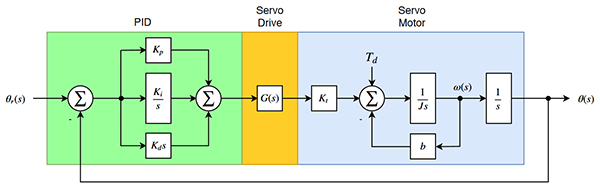
The PID operates on the position error and outputs a torque command to the servo driver. Three gains need to be adjusted in the PID controller (K_p, K_i and K_d). They act on the error between the desired and present position.


The signal output from the PID is


The ways of selecting the gains for the PID controller can be accomplished by, following the Ziegler and Nichols method based on setting K_i and K_d to zero, analyzing the system's step response while slowly increasing K_p until the shaft position oscillates and recording both K_p and the oscillation frequency. That data can then be used to calculate the final values of K_p and K_i and K_d. This last approach doesn't usually yield many benefits to a high-performance servo system. The settling time can generally be further improved.

PIV

An easier-to-tune alternative to the PID that has a better predicted system response is the PIV topology (Fig. 2.2). This controller combines a position and velocity loop. A velocity correction command results from the position error multiplied by K_p. K_i now operates directly on the velocity error as opposed to the position error in the PID. K_d is replaced by K_v.
To accurately use this topology, a good knowledge of the motor velocity is required. To tune this system, two control parameters are needed: The bandwidth (BW) and damping ratio(ζ ). An estimate of the rotor and load moment of inertia j and damping constant b are also required. Higher bandwidth is related to quicker rise and settling times while damping pertains mainly to overshoot. The K_p, K_i and K_v, constants can be calculated from equations 2.4, 2.5 and 2.6.


Feed-Forward

To accomplish near-zero following and tracking errors, feed-forward is often used in combination with a PID or PIV loop. For this topology, the controller needs access to a position θ_r(s), velocity ω_r(s), and acceleration α_r(s) commands (Fig. 2.3). Total inertia and damping ration estimates should also be available.
To calculate the estimated torque needed to make the desired motion, equation 2.7 is used.


Feed-forward control reduces settling time and minimizes overshoot. In any case, to increase the velocity estimation accuracy, an encoder with enough resolution for the feedback is also required.

Parameter Estimation

RC servo motors are comprised of three main components: a DC motor, driving circuitry with a potentiometer encoder for position feedback, and a gear reduction system. When modeling the controller, certain parameters from the DC motor need to be appropriately measured or estimated for improved control. They can be extracted from the transitory response to a step on the input and steady-state response for different input voltages. The model in Fig. 2.4 can be defined by equation 2.8, where i_a is the armature current and the voltage V is the sum of the voltage drop across the equivalent resistance R, equivalent inductance L, and back electromotive force e.


Equation 2.9 shows the resulting torque T_r as it relates to the developed torque T_d, static friction torque T_c and viscous friction bθ.


The following equations express the relationship between developed torque T_d and current i_a (2. 10), back electromotive force e and angular velocity ω(2.11), and load torque T_L with the moment of inertia J and angular acceleration ω (2.12).


From these equations, we can obtain the angular acceleration ω which can then be discretized into where △T is the sampling time.


Equation 2.15 can then be attained by minimizing the sum of the absolute error between the estimated (2.14) and actual transitory response, assuming zero inductive voltage drop across L and initial known values of T_c and K.


Where:


In steady state ω=c/d resulting in:

By repeating the procedure starting from an estimated value for R to obtain Tc and K and replacing them with the new estimations to get R back, the parameters will converge to the real values.